Trapezoidal Methods for Solving ODE Systems
With the trapezoidal rule we can integrate ordinary differential equations (ODEs) with second-order global accuracy while retaining good stability properties.
1. The Method
Given $\dot{\mathbf x}=f(t,\mathbf x)$ and step–size $h=t_{n+1}-t_n$
Implicit trapezoidal
[ \mathbf x_{n+1}= \mathbf x_n + \frac{h}{2}\Bigl(f\bigl(t_n,\mathbf x_n\bigr)+f\bigl(t_{n+1},\mathbf x_{n+1}\bigr)\Bigr). ]
Because $\mathbf x_{n+1}$ appears on both sides, we solve a nonlinear system (here with scipy.optimize.fsolve).
Modified (predictor–corrector) trapezoidal
- Predictor: $\mathbf{x}_{n+1}^{*}= \mathbf x_n + h\,f(t_n,\mathbf x_n)$ (Explicit Euler)
- Corrector: $\mathbf x_{n+1}= \mathbf x_n + \dfrac{h}{2}\bigl(f(t_n,\mathbf x_n)+f(t_{n+1}, \mathbf x_{n+1}^{*})\bigr)$
This avoids solving an implicit equation yet keeps second-order accuracy.
2. Example Problem
We reuse the linear three-component system from the previous post:
[
\begin{aligned}
\dot x_1 &= -\tfrac12 x_1,
\dot x_2 &= \tfrac12 x_1-\tfrac14 x_2,
\dot x_3 &= \tfrac14 x_2-\tfrac16 x_3,
\end{aligned}\qquad t\in[0,1], \quad \mathbf x(0)=(1,1,1).
]
import numpy as np
from scipy.optimize import fsolve

h   = 0.01
t   = np.arange(0, 1+h, h)
x0  = np.array([1., 1., 1.])

def model(x, t):
    x1, x2, x3 = x
    return np.array([
        -0.5*x1,
        0.5*x1 - 0.25*x2,
        0.25*x2 - (1/6)*x3
    ])
2.1 Implicit trapezoidal
def explict_trapz(F, c0,  t):
    X = np.zeros((len(t), len(c0)))
    X[0] = c0
    for n in range(len(t) - 1):
        f1 = lambda x: x - X[n] - 0.5*h*(F(X[n], t[n]) + F(x, t[n+1]))
        X[n+1] = fsolve(f1, X[n])
    return X

imp_trap = explict_trapz(model, x0, t)
ip1_t = imp_trap[:, 0]
ip2_t = imp_trap[:, 1]
ip3_t = imp_trap[:, 2]
print()
print()
print("\t      =======================================================================================")
print(f"\t   ** Plot of Exact solution, Approximate solution, and the error Using Implict Trapizoidal **")
print("\t      =======================================================================================\n")

plot(t, x1t(t), ip1_t, 'Modified trapzoidal', "Exact VS Implict Trapizoidal for x1", abs(x1t(t) - ip1_t))
plot(t, x2t(t), ip2_t, 'Modified trapzoidal', "Exact VS Implict Trapizoidal for x2", abs(x2t(t) - ip2_t))
plot(t, x3t(t), ip3_t, 'Modified trapzoidal', "Exact VS Implict Trapizoidal for x3", abs(x3t(t) - ip3_t))
Running the code produces the following absolute-error plots against the analytic solution:
2.2 Modified trapezoidal
def modified_trapz(F, c0, t):
    X = np.zeros((len(t), len(c0)))
    X[0] = c0
    for n in range(len(t) - 1):
        Xp = X[n] + h*F(X[n], t[n])
        X[n+1] = X[n] + 0.5*h*(F(X[n], t[n]) + F(Xp, t[n+1]))
    return X

md_tr = modified_trapz(model, x0, t)
md1_tr = md_tr[:,0]
md2_tr = md_tr[:,1]
md3_tr = md_tr[:,2]
print()
print()
print("\t =======================================================================================")
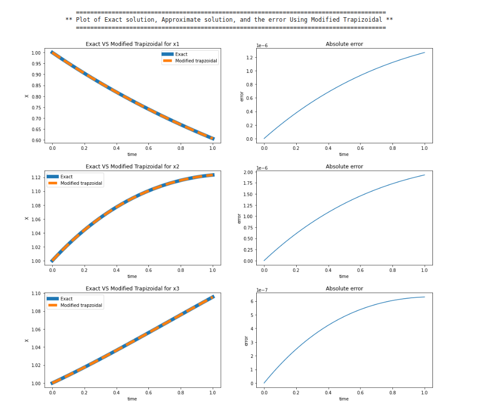
print(f"\t ** Plot of Exact solution, Approximate solution, and the error Using Modified Trapizoidal **")
print("\t =======================================================================================\n")
plot(t, x1t(t), md1_tr, 'Modified trapzoidal', "Exact VS Modified Trapizoidal for x1", abs(x1t(t) - md1_tr))
plot(t, x2t(t), md2_tr, 'Modified trapzoidal', "Exact VS Modified Trapizoidal for x2", abs(x2t(t) - md2_tr))
plot(t, x3t(t), md3_tr, 'Modified trapzoidal', "Exact VS Modified Trapizoidal for x3", abs(x3t(t) - md3_tr))
Running the code produces the following absolute-error plots against the analytic solution:
3. Take-aways
- Both schemes are second order.
- The fully implicit version is A-stable and therefore more robust for stiff problems.
- The predictor-corrector variant trades some stability for computational simplicity.
You can download the full notebook from here.