Runge–Kutta Methods: 2nd- and 4th-Order Schemes
Runge–Kutta (RK) methods provide a family of explicit single-step integrators that achieve higher-order accuracy without needing derivatives beyond $f(t,x)$.
1. Recap of the idea
Starting from the Taylor expansion we construct weighted averages of slopes $k_i$.
1.1 2nd-order midpoint (RK2)
[
\begin{aligned}
k_1 &= h\,f(t_n,x_n),
k_2 &= h\,f\bigl(t_n+\tfrac{h}{2},\,x_n+\tfrac{k_1}{2}\bigr),
x_{n+1} &= x_n + k_2.
\end{aligned}
]
def sec_rangeKuta(F, c0, t, h):
    X = np.zeros((len(t), len(c0)))
    X[0] = c0
    for n in range(len(t)-1):
        k1 = h*F(X[n], t[n])
        k2 = h*F(X[n] + 0.5*k1, t[n] + 0.5*h)
        X[n+1] = X[n] + k2
    return X

sec_rng = sec_rangeKuta(model, x0, t, h)
sec1_rn = sec_rng[:,0]
sec2_rn = sec_rng[:,1]
sec3_rn = sec_rng[:,2]
print()
print()
print("\t =======================================================================================")
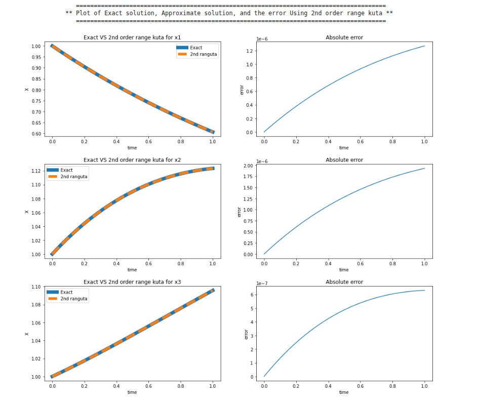
print(f"\t ** Plot of Exact solution, Approximate solution, and the error Using 2nd order range kuta **")
print("\t =======================================================================================\n")
plot(t, x1t(t), sec1_rn, '2nd ranguta', "Exact VS 2nd order range kuta for x1", abs(x1t(t) - sec1_rn))
plot(t, x2t(t), sec2_rn, '2nd ranguta', "Exact VS 2nd order range kuta for x2", abs(x2t(t) - sec2_rn))
plot(t, x3t(t), sec3_rn, '2nd ranguta', "Exact VS 2nd order range kuta for x3", abs(x3t(t) - sec3_rn))
Running the code produces the following absolute-error plots against the analytic solution:
1.2 Classic 4th-order (RK4)
[
\begin{aligned}
k_1 &= h\,f(t_n,x_n),
k_2 &= h\,f\bigl(t_n+\tfrac{h}{2},\,x_n+\tfrac{k_1}{2}\bigr),
k_3 &= h\,f\bigl(t_n+\tfrac{h}{2},\,x_n+\tfrac{k_2}{2}\bigr),
k_4 &= h\,f(t_n+h,\,x_n+k_3),
x_{n+1} &= x_n + \tfrac16\bigl(k_1+2k_2+2k_3+k_4\bigr).
\end{aligned}
]
def forth_rangeKuta(F, c0, t, h):
    X = np.zeros((len(t), len(c0)))
    X[0] = c0
    for n in range(len(t)-1):
        k1 = h*F(X[n], t[n])
        k2 = h*F(X[n] + 0.5*k1, t[n] + 0.5*h)
        k3 = h*F(X[n] + 0.5*k2, t[n] + 0.5*h)
        k4 = h*F(X[n] + k3, t[n] + h)
        X[n+1] = X[n] + 1/6*(k1 + 2*k2 + 2*k3 + k4)
    return X

frz_rng = forth_rangeKuta(model, x0, t, h)
frz1_rng = frz_rng[:,0]
frz2_rng = frz_rng[:,1]
frz3_rng = frz_rng[:,2]
print()
print()
print("\t =======================================================================================")
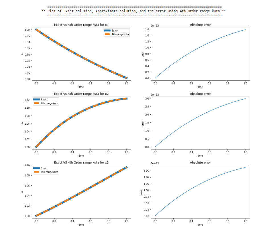
print(f"\t ** Plot of Exact solution, Approximate solution, and the error Using 4th Order range kuta **")
print("\t =======================================================================================\n")
plot(t, x1t(t), frz1_rng, '4th rangekuta', "Exact VS 4th Order range kuta for x1", abs(x1t(t) - frz1_rng))
plot(t, x2t(t), frz2_rng, '4th rangekuta', "Exact VS 4th Order range kuta for x2", abs(x2t(t) - frz2_rng))
plot(t, x3t(t), frz3_rng, '4th rangekuta', "Exact VS 4th Order range kuta for x3", abs(x3t(t) - frz3_rng))
Running the code produces the following absolute-error plots against the analytic solution:
3. Discussion
- RK4 is the workhorse of non-stiff ODE solvers, excellent accuracy versus cost.
- Higher-order explicit RK methods exist, but RK4 is usually sufficient.
- For stiff systems combine RK ideas with implicitness (e.g. diagonally implicit RK).
You can download the full notebook from here. Feel free to adapt the code to your own problems!