Explict Euler method for Ordinary Differential Equations(ODEs) using Python

Theory

Let $t_k$ be a partition of $[a,b]$ such that $a=t_0<t_1<\cdots<t_{N-1}<t_{N}=b$ and $;H$ be the constant length of the $k$ -th subinterval $H = t_k - t_{k-1}$ . Let us consider the initial value problem.

$\begin{equation} \begin{cases} y' = F(y, t), & \quad \text{on } [a, b]\\\\ y(a) = c, \end{cases} \end{equation}$

We can compute $y_{k+1}$ using the iterative equation. $y_{k+1} = y_k + HF(y_k, t_k)$

And this iterative equation is called the Explict euler formula.

Implementation and Plots

Now let us see the implementation of explict euler formula using python.

  """
It takes partition boundaries-"a,b", the differential equation-"F", initial values-'c', and the step size-'h'
as argument and returns the numerical solution.
"""
def euler_explict(a, b, F, c, h):
    N = int((b-a)/h + 1)
    t = np.linspace(a, b, N)
    y = np.zeros((len(t), len(c0)))
    y[0] = c
    for k in range(N):
        y[k+1] = y[k] + h*F(y[k], t[k])
    return y               

Example

Write code to solve the following system of ordinary differential equations

$\begin{cases} \frac{dx_1}{dt} = -\frac{1}{2}x_1\\\\ \frac{dx_2}{dt} = \frac{1}{2}x_1-\frac{1}{4}x_2 & \quad \text{ on } [0,4]\\\\ \frac{dx_3}{dt} = \frac{1}{4}x_2-\frac{1}{6}x_3 \end{cases}$

Subject to the initial conditions $x_1(0) = 1, x_2(0) = 1, x_3(0) = 1$

The exact solution of the above system of ODEs is given by

$\begin{cases} x_1(t) = e^{-t/2}\\ x_2(t)= -2e^{-t/2}+3e^{-t/4}\\ x_3(t) = \dfrac{3}{2}e^{-t/2} - 9e^{-t/4} + \dfrac{17}{2}e^{-t/6} \end{cases}$

Let us implement the above system of ode and compire with the exact solution by plotting.

# import required libraries
import numpy as np
import matplotlib.pyplot as plt
from scipy.optimize import fsolve
from scipy.integrate import odeint
import warnings
warnings.simplefilter("ignore")

Define the exact solutions

x1t = lambda t : np.exp(-t*0.5)
x2t = lambda t : -2*np.exp(-t*0.5) + 3*np.exp(-t*0.25)
x3t = lambda t: 1.5*np.exp(-t*0.5) - 9*np.exp(-t*0.25) + 8.5*np.exp(-t*1/6)

Let us define a function to plot the solutions and the error.

def plot(time, exact, approximate, label, title, abs_er):
    
    # plot for exact vs approximation
    plt.figure(figsize=(16, 4))
    plt.subplot(1,2,1)
    plt.plot(time, exact, linewidth = 8, label="Exact")
    plt.plot(time, approximate, linewidth = 6, linestyle='--', label=label)
    plt.xlabel('time')
    plt.ylabel('X')
    plt.title(title)
    plt.legend()
    
    
    # plot for absolute error
    plt.subplot(1,2,2)
    plt.plot(time, abs_er)
    plt.title('Absolute error')
    plt.xlabel('time')
    plt.ylabel("error")

Let us define the system of the differential equation

# defining the system of the differential equation
def model(x, t):
    x1, x2, x3 = x
    dx1dt = -0.5*x1
    dx2dt = 0.5*x1 - 0.25*x2
    dx3dt = 0.25*x2 - (1/6)*x3
    return np.array([dx1dt, dx2dt, dx3dt])

And assigne the values of the parametrs and call our function.

a, b = [0, 4]
h = 0.01
c = np.array([1, 1, 1])
euler = euler_explict(a, b, model, c, h) # calling our function
x_e1 = euler[:,0]
x_e2 = euler[:,1]
x_e3 = euler[:,2]

Now let us plot it.

print()
print()
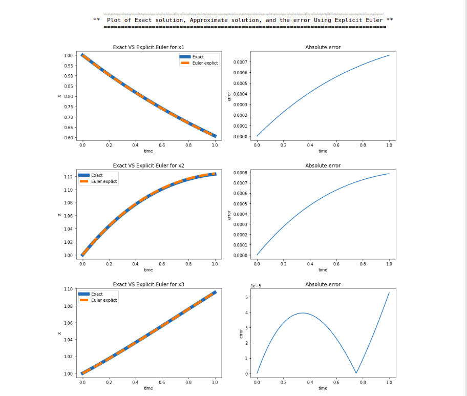
print("\t      =================================================================================")
print(f"\t   **  Plot of Exact solution, Approximate solution, and the error Using Explicit Euler **")
print("\t      ==================================================================================\n")

plot(t, x1t(t), x_e1, 'Euler explict', "Exact VS Explicit Euler for x1", abs(x1t(t) - x_e1))
plot(t, x2t(t), x_e2, 'Euler explict', "Exact VS Explicit Euler for x2", abs(x2t(t) - x_e2))
plot(t, x3t(t), x_e3, 'Euler explict', "Exact VS Explicit Euler for x3", abs(x3t(t) - x_e3))

euler_explicit